Introduction
Since this is my first post, I would like to play around with some fun data and show some multivariate analysis. In 1994, Electronics Arta (EA) published “FIFA International Soccer,” a game that was welcomed by soccer fans in Europe. Year after year, EA released new versions of this game, reaching substantial improvements in graphics and AI behavior. Finally, after 2002, FIFA’s sales exceeded the most played soccer game at the moment, Pro Evolution Soccer. Since then, FIFA is considered the leading soccer game with huge revenues. 1
During the past several years, EA made a vital effort to improve the game’s reality, especially in physics’ details and players facial and behavioral features. Part of this exercise was the opportunity to identify the strengths and weaknesses of each player by quantifying different attributes of each player. Each player has some characteristics, physical, behavioral and technical, that, at some level, could determine the position of this player. Let’s use some multivariate analysis to determine the latter.
Objective
Our primary objective is to build a model that predicts the player’s position based on his attributes. Why? Well, it can help, in the future, to create new players based on their characteristics and position them in the best place on the field. In other words, it could help us identify more easily the ideal position for a player.
Diving into the data
First, we use the FIFA 2018 dataset at Kaggle which has all the information for each player, including attributes, photos, nationality, among others. In this case we will work with just attributes and position of each player. Although a player can play at different positions, as a first exercise we will just use the first position listed in this variable. Here is a good explanation of soccer positions. But first, lets take a look at the database:
library(boot)
library(MASS)
library(datasets)
library(dplyr)
library(knitr)
library(mvnmle)
library(FactoClass)
library(mclust)
library(readr)
library(caTools)
library(factoextra)
library(ICSNP)
library(FactoMineR)
library(ggpubr)
base <- read_csv("CompleteDataset.csv")

# Let's take a look to the complete database
glimpse(base)
## Observations: 17,981
## Variables: 75
## $ X1                    <dbl> 0, 1, 2, 3, 4, 5, 6, 7, 8, 9, 10, 11, 12...
## $ Name                  <chr> "Cristiano Ronaldo", "L. Messi", "Neymar...
## $ Age                   <dbl> 32, 30, 25, 30, 31, 28, 26, 26, 27, 29, ...
## $ Photo                 <chr> "https://cdn.sofifa.org/48/18/players/20...
## $ Nationality           <chr> "Portugal", "Argentina", "Brazil", "Urug...
## $ Flag                  <chr> "https://cdn.sofifa.org/flags/38.png", "...
## $ Overall               <dbl> 94, 93, 92, 92, 92, 91, 90, 90, 90, 90, ...
## $ Potential             <dbl> 94, 93, 94, 92, 92, 91, 92, 91, 90, 90, ...
## $ Club                  <chr> "Real Madrid CF", "FC Barcelona", "Paris...
## $ `Club Logo`           <chr> "https://cdn.sofifa.org/24/18/teams/243....
## $ Value                 <chr> "€95.5M", "€105M", "€123M", "€97M", "€61...
## $ Wage                  <chr> "€565K", "€565K", "€280K", "€510K", "€23...
## $ Special               <dbl> 2228, 2154, 2100, 2291, 1493, 2143, 1458...
## $ Acceleration          <chr> "89", "92", "94", "88", "58", "79", "57"...
## $ Aggression            <chr> "63", "48", "56", "78", "29", "80", "38"...
## $ Agility               <chr> "89", "90", "96", "86", "52", "78", "60"...
## $ Balance               <chr> "63", "95", "82", "60", "35", "80", "43"...
## $ `Ball control`        <chr> "93", "95", "95", "91", "48", "89", "42"...
## $ Composure             <chr> "95", "96", "92", "83", "70", "87", "64"...
## $ Crossing              <chr> "85", "77", "75", "77", "15", "62", "17"...
## $ Curve                 <chr> "81", "89", "81", "86", "14", "77", "21"...
## $ Dribbling             <chr> "91", "97", "96", "86", "30", "85", "18"...
## $ Finishing             <chr> "94", "95", "89", "94", "13", "91", "13"...
## $ `Free kick accuracy`  <chr> "76", "90", "84", "84", "11", "84", "19"...
## $ `GK diving`           <chr> "7", "6", "9", "27", "91", "15", "90", "...
## $ `GK handling`         <chr> "11", "11", "9", "25", "90", "6", "85", ...
## $ `GK kicking`          <chr> "15", "15", "15", "31", "95", "12", "87"...
## $ `GK positioning`      <dbl> 14, 14, 15, 33, 91, 8, 86, 8, 7, 5, 7, 1...
## $ `GK reflexes`         <chr> "11", "8", "11", "37", "89", "10", "90",...
## $ `Heading accuracy`    <chr> "88", "71", "62", "77", "25", "85", "21"...
## $ Interceptions         <chr> "29", "22", "36", "41", "30", "39", "30"...
## $ Jumping               <chr> "95", "68", "61", "69", "78", "84", "67"...
## $ `Long passing`        <chr> "77", "87", "75", "64", "59", "65", "51"...
## $ `Long shots`          <chr> "92", "88", "77", "86", "16", "83", "12"...
## $ Marking               <chr> "22", "13", "21", "30", "10", "25", "13"...
## $ Penalties             <chr> "85", "74", "81", "85", "47", "81", "40"...
## $ Positioning           <chr> "95", "93", "90", "92", "12", "91", "12"...
## $ Reactions             <chr> "96", "95", "88", "93", "85", "91", "88"...
## $ `Short passing`       <chr> "83", "88", "81", "83", "55", "83", "50"...
## $ `Shot power`          <chr> "94", "85", "80", "87", "25", "88", "31"...
## $ `Sliding tackle`      <chr> "23", "26", "33", "38", "11", "19", "13"...
## $ `Sprint speed`        <chr> "91", "87", "90", "77", "61", "83", "58"...
## $ Stamina               <chr> "92", "73", "78", "89", "44", "79", "40"...
## $ `Standing tackle`     <chr> "31", "28", "24", "45", "10", "42", "21"...
## $ Strength              <chr> "80", "59", "53", "80", "83", "84", "64"...
## $ Vision                <chr> "85", "90", "80", "84", "70", "78", "68"...
## $ Volleys               <chr> "88", "85", "83", "88", "11", "87", "13"...
## $ CAM                   <dbl> 89, 92, 88, 87, NA, 84, NA, 88, 83, 81, ...
## $ CB                    <dbl> 53, 45, 46, 58, NA, 57, NA, 47, 72, 46, ...
## $ CDM                   <dbl> 62, 59, 59, 65, NA, 62, NA, 61, 82, 52, ...
## $ CF                    <dbl> 91, 92, 88, 88, NA, 87, NA, 87, 81, 84, ...
## $ CM                    <dbl> 82, 84, 79, 80, NA, 78, NA, 81, 87, 71, ...
## $ ID                    <dbl> 20801, 158023, 190871, 176580, 167495, 1...
## $ LAM                   <dbl> 89, 92, 88, 87, NA, 84, NA, 88, 83, 81, ...
## $ LB                    <dbl> 61, 57, 59, 64, NA, 58, NA, 59, 76, 51, ...
## $ LCB                   <dbl> 53, 45, 46, 58, NA, 57, NA, 47, 72, 46, ...
## $ LCM                   <dbl> 82, 84, 79, 80, NA, 78, NA, 81, 87, 71, ...
## $ LDM                   <dbl> 62, 59, 59, 65, NA, 62, NA, 61, 82, 52, ...
## $ LF                    <dbl> 91, 92, 88, 88, NA, 87, NA, 87, 81, 84, ...
## $ LM                    <dbl> 89, 90, 87, 85, NA, 82, NA, 87, 81, 79, ...
## $ LS                    <dbl> 92, 88, 84, 88, NA, 88, NA, 82, 77, 87, ...
## $ LW                    <dbl> 91, 91, 89, 87, NA, 84, NA, 88, 80, 82, ...
## $ LWB                   <dbl> 66, 62, 64, 68, NA, 61, NA, 64, 78, 55, ...
## $ `Preferred Positions` <chr> "ST LW", "RW", "LW", "ST", "GK", "ST", "...
## $ RAM                   <dbl> 89, 92, 88, 87, NA, 84, NA, 88, 83, 81, ...
## $ RB                    <dbl> 61, 57, 59, 64, NA, 58, NA, 59, 76, 51, ...
## $ RCB                   <dbl> 53, 45, 46, 58, NA, 57, NA, 47, 72, 46, ...
## $ RCM                   <dbl> 82, 84, 79, 80, NA, 78, NA, 81, 87, 71, ...
## $ RDM                   <dbl> 62, 59, 59, 65, NA, 62, NA, 61, 82, 52, ...
## $ RF                    <dbl> 91, 92, 88, 88, NA, 87, NA, 87, 81, 84, ...
## $ RM                    <dbl> 89, 90, 87, 85, NA, 82, NA, 87, 81, 79, ...
## $ RS                    <dbl> 92, 88, 84, 88, NA, 88, NA, 82, 77, 87, ...
## $ RW                    <dbl> 91, 91, 89, 87, NA, 84, NA, 88, 80, 82, ...
## $ RWB                   <dbl> 66, 62, 64, 68, NA, 61, NA, 64, 78, 55, ...
## $ ST                    <dbl> 92, 88, 84, 88, NA, 88, NA, 82, 77, 87, ...
There are 75 variables and 17,981 players in this dataset. We can see, from the function glimpse of dplyr package, that the attributes variables (starting at Acceleration and finishing at Volleys) are not as numeric variables but as characters. These variables are numeric variables between 0 and 100, where 100 describes that the player reaches the maximun of this attribute. If you want to see each one of these in detail you can see here or here.
Another critical thing to notice is that in this exercise we will not take into account the variables that describe the ratings at each position, we just want to observe, for now, the relationship between the attributes and the position of each player.
Having that clear, let’s make some adjustments to the database. First, we will take the variables we are interested in: Name, Nationality, Attributes, ID and Position. Then, we need to obtain the first position in the variable Position. Followed by the transformation of the attributes to just numeric variables and holding them in a data frame named fifa.
# Select variables : Name, Nationality, Attributes, ID, Position
fifa <- base %>% select(Name, Nationality, 14:47, ID, Position = `Preferred Positions`)

# Split the Position variable and take just the first one
fifa$Position <- lapply(fifa$Position, function(x) strsplit(x, split = " ")[[1]][1])
fifa$Position <- as.character(fifa$Position)

# Take attributes and convert them to integers
fifa[,3:37] <- data.frame(lapply(fifa[,3:37], as.numeric))
Since we want to predict the position of the player based on the attributes, we need to train a model and then test it. What we will make next is divide the database fifa into two datasets, one for training (train with 70% of the players) and the other one for testing (test with the remaining 30%).
# Set the seed to make in replicable and select 70% for training
set.seed(123)
fifa$base <- sample.split(fifa$Name, SplitRatio = 0.7)
train <- fifa %>% filter(base == TRUE) %>% select(-base)
train <- train[complete.cases(train),]
test <- fifa %>% filter(base == FALSE) %>% select(-base)
test <- test[complete.cases(test),]

# We just want the numeric data for each database
train.x <- train %>% select(-Name, -Position, -Nationality, -Position2, -Position3)
train.x <- data.frame(lapply(train.x, as.numeric))
test.x <- test %>% select(-Name, -Position, -Nationality, -Position2, -Position3)
test.x <- data.frame(lapply(test.x, as.numeric))
Figure 1 helps us understand the behaviour of each attribute between players. For instance, a majority has low levels of Goalkeepers attributes, which is evident since just a few players play in this position. Contrarily, many players have attributes’ levels ranging between 50 and 75, with few having more than these levels. Figure 2 illustrates these differences with more details. One can see that Defenders and Strickers (B and ST, respectively in the figure) have specific attributes related to their position, like Sliding tackles, Strength, Standing tackle, etc. in the case of Defenders, or Finishing, Dribbling, etc. On the contrary, Midfielders have more similar attributes, which makes them more capable of playing in any position.
ggplot(data = reshape2::melt(train.x[,-35]), aes(value)) + geom_density(aes(colour = variable), alpha = 0.2) + labs(x = "Attribute's level", y = "Density", colour = "Attribute") + theme_gray()
## No id variables; using all as measure variables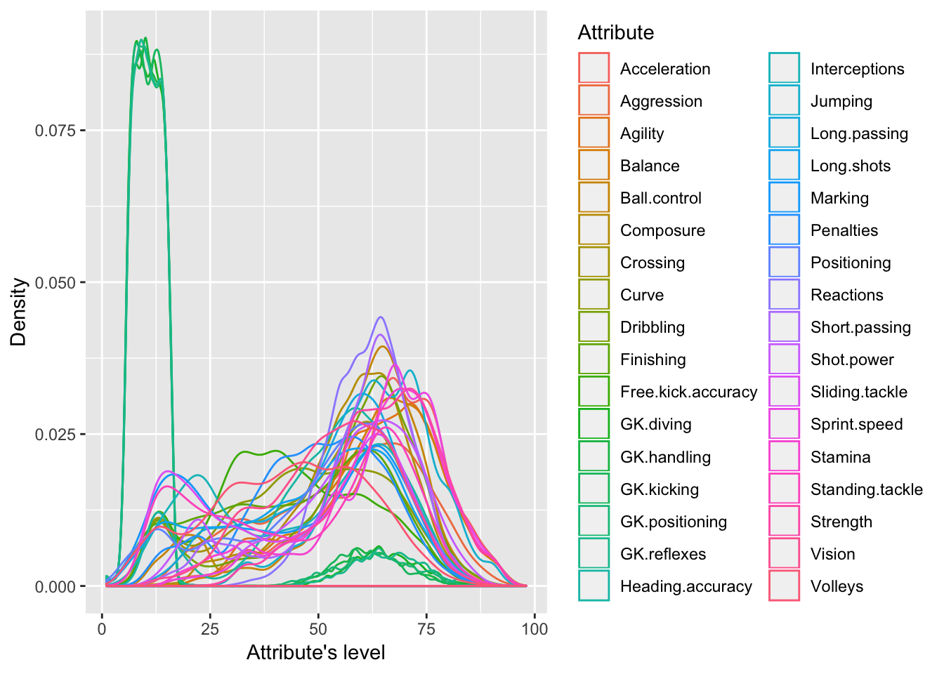
Figure 1: Density distributions of attributes
train %>% select(-Name, -Position, -Nationality, -ID, -Position3) %>% reshape2::melt(c("Position2")) %>% ggplot(aes(value)) + geom_density(aes(colour = variable), alpha = 0.2) + labs(x = "Attribute's level", y = "Density", colour = "Attribute") + theme_gray() + facet_grid(. ~ Position2)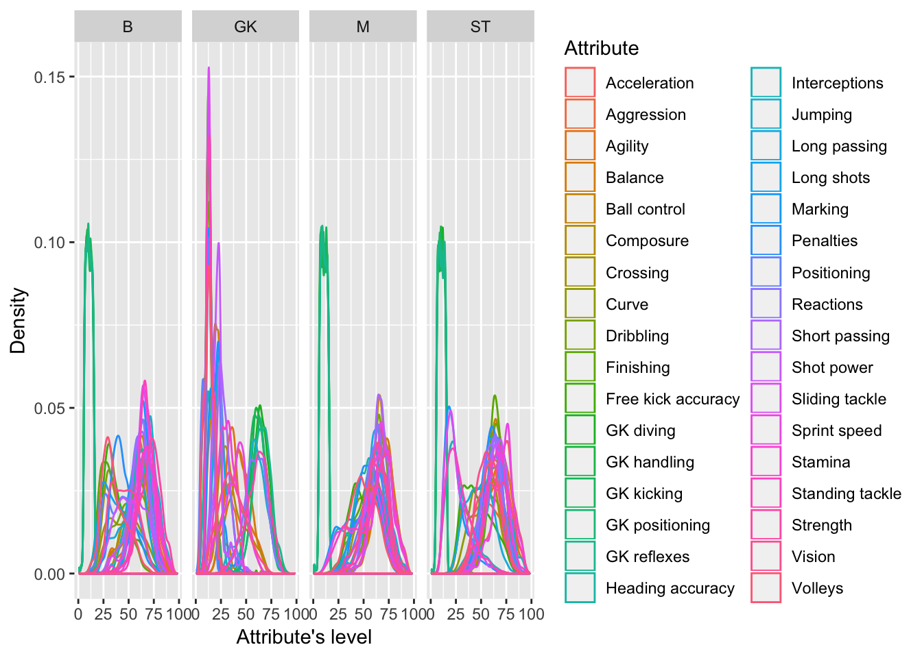
Figure 2: Density distributions of attributes by position
The previous figures allow us to predict that Goalkeepers, Defenders and Strickers should differentiate more clearly when applying multivariate models, while Midfielders will have less variance; therefore, they should appear to get mixed with the last two positions. To prove the latter, we are going to use the first two components after applying PCA with, and then without, Goalkeepers. In Figure 3 one can see that Goalkeepers have specific qualities that are not shared with the other players, clustering the low-right quadrant of the graph. On the contrary, the Defenders (B), Midfielders (M), and Strickers (ST) share some common attributes, especially the last two positions.
pca <- train %>% select(-Name, -Position, -Nationality, -ID, -Position3) %>% PCA(quali.sup = 35, graph = FALSE)
fviz_pca_biplot(pca, geom.ind = "point", habillage = 35, repel = TRUE, title = "PCA - Attributes", alpha.ind = 0.5, alpha.var = 0.5, col.var = "black") %>% ggpar(legend.title = "Position", legend = "bottom", palette = "jco")
pca_nogk <- train %>% filter(!Position2 %in% c("GK")) %>% select(-Name, -Position, -Nationality, -ID, -Position3) %>% PCA(quali.sup = 35, graph = FALSE)
fviz_pca_biplot(pca_nogk, geom.ind = "point", habillage = 35, repel = TRUE, title = "PCA - Attributes without GK", alpha.ind = 0.5, alpha.var = 0.5, col.var = "black", addEllipses = TRUE) %>% ggpar(legend.title = "Position", legend = "bottom", palette = "jco")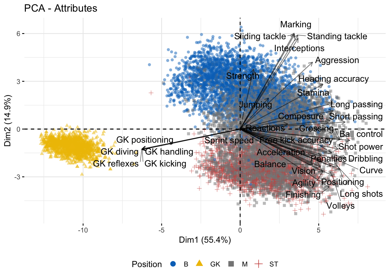
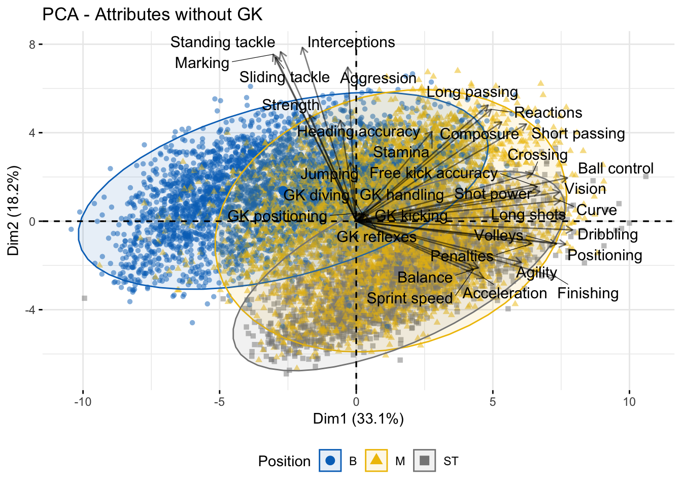
Figure 3: PCA Biplot
To understand better the relationship between variables and positions we could use a barplot with the contribution of each variable to the first component is the perfect way to understand it. The Figure 4 shows the results when Goalkeepers are taken into account. The significant contributions to the first component are Ball control, Dribbling, Short passing, Crossing, Positioning, Shot power, and Goalkeepers’ attributes. With the biplot and the barplot, one can see that the attributes contrast between specific Goalkeepers attributes and non-specific ones, this implies that the first component “divides” the axes between Goalkeepers and the other positions. On the other hand, the second component seems to divide the Defenders from the Strikers and some Midfielders, as can be seen from both the biplot and the barplot.
fviz_contrib(pca, title = "PCA - Attributes", choice = "var") %>% ggpar(palette = "jco")
fviz_contrib(pca, title = "PCA - Attributes", choice = "var", axes = 2) %>% ggpar(palette = "jco")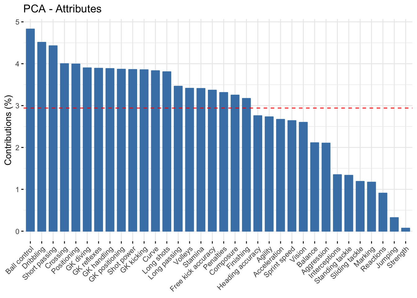
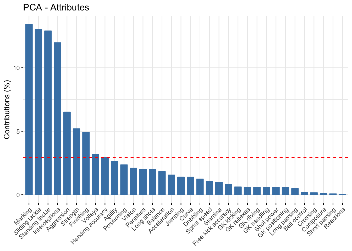
Figure 4: PCA Variables
From the second biplot in Figure 3, one can notice the division the Midfielders have between the attributes shared with Defenders and Strickers. In Figure 5 the PCA is done exclusively for the Midfielders but taking into account the different positions that exist in the game. One can see that the CDMs, or Central Defensive Midfielders, are located at the upper part of the second axes, which has a significant contribution from the defensive attributes. CMs or Central Midfielders are as well at a higher position than the other positions. By contrast, the rest of Midfielders’ positions are related to attributes like Ball Control, Finishing, Agility, Long shots, etc. All of these highlights means that there essential differences between the Midfielders positions that attack and defence.
pca_m <- train %>% filter(Position %in% c("M", "CAM", "CDM", "CM", "LM", "RM")) %>% select(-Name, -Position2, -Nationality, -ID, -Position3) %>% PCA(quali.sup = 35, graph = FALSE)
fviz_pca_biplot(pca_m, geom.ind = "point", habillage = 35, repel = TRUE, title = "PCA - Attributes for Midfielders", alpha.ind = 0.5, alpha.var = 0.5, col.var = "black", addEllipses = TRUE) %>% ggpar(legend.title = "Position", legend = "bottom", palette = "jco")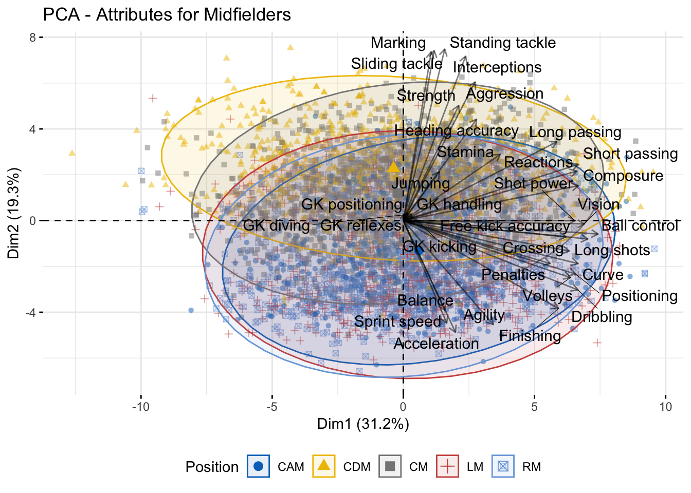
Figure 5: PCA for the Midfielders
Although we can get deeper into the data and produce several discoveries (nothing compared to a shipwreck), the purpose of this exercise was to predict the position based on the attributes. To accomplish that, I selected the Discriminant Analysis through eigenvalue decomposition, which is in the package mclust (for more information you visit the mclust paper). We will use the Gaussian finite mixture model for discriminant analysis where a single Gaussian term models each class but assuming different covariances with-in class. In other words, we will use the Eigenvalue Decomposition Discriminant Analysis, named “EDDA”, but assuming a within-class covariance matrix (“VVV”).
fifa_clust <- MclustDA(train.x[,-35], train$Position2, modelType = "EDDA", modelNames = "VVV")
s_fifa_clust <- summary(fifa_clust, parameters = TRUE, newdata = test.x[, -35])
Using the command MclustDA from the package mclust we estimate the model with the train data, but excluding the ID column. After applying it, we can view the result using the summary method of the object of class MclustDA, and it has the option to include the test data with the newdata = argument. It will print many things about the model, but what we are mostly interested in are the error rate and the table that presents the original class and the predicted one. The error can be accessed by selecting the err object of the list produced by the summary command. The result in this model is: s_fifa_clust2$err = 0.187.
The level of the error is a little high, but it is mainly fault of the common attributes shared by the Midfielders with Defenders and Strickers. The latter can be seen in the next code’s chunk exit, where the misclassification of the Midfielders is higher than the rest of positions. In conclusion, this model could help the objective of trying to anticipate the best position of a player, although it could be improved more to get better results (I hope to do this soon).
# Class vs. Predicted
s_fifa_clust$tab
##      Predicted
## Class    B   GK    M   ST
##    B  3210    0  401   11
##    GK    0 1377    0    0
##    M   679    0 3457  726
##    ST   18    0  433 1803
Twitter
Reddit
LinkedIn
Email